Some examples of lenstool usage on Jupyter Notebook

The SIS model (Singular Isothermal Sphere)

In this notebook we will showcase lensing modelling with Lenstool using the SIS model.

from astropy.io import fits
import matplotlib.pyplot as plt
from astropy.wcs import WCS
from astropy.table import Table
from matplotlib.patches import Ellipse
from matplotlib.patches import Circle
import os
import matplotlib.cm as cm
from matplotlib.colors import Normalize
import numpy
import lenstool
from lenstool.potentials import sis

---------------------------------------------------------------------------
ModuleNotFoundError                       Traceback (most recent call last)
Cell In[1], line 2
      1 from astropy.io import fits
----> 2 import matplotlib.pyplot as plt
      3 from astropy.wcs import WCS
      4 from astropy.table import Table

ModuleNotFoundError: No module named 'matplotlib'

lt = lenstool.Lenstool()
lt.add_lens(sis(0.,0.,0.3,800))
lt.set_cosmology(70, 0.3, 0.7, -1)
lt.set_field(50)
lt.set_grid(1000, 1)

The inputs

We will first define the lens model. In this example, the lens is a single SIS potential. It is centered at (0,0) and has a redshift of 0.3.

lt.get_lenses()

Table length=1

type	n	x	y	z
int64	str1	float64	float64	float64
1	1	0.0	0.0	0.3

The source definition

The source properties are coordinates in arcsec, size, redshift, orientation angle and magnitude (brightness). These parameters must be given directly in the code . Here we study a circular source of redshift 1 and magnitude 20.

tab = Table(names=['n','x','y','a','b','theta','z','mag'], dtype=['str',*['float',]*7])
tab.add_row(['1a', 0.6789067, -9.7, 3.5, 3.5, 0, 1.0, 20])
lt.set_sources(tab)
lt.get_sources()

Table length=1

n	x	y	a	b	theta	z	mag
str2	float64	float64	float64	float64	float64	float64	float64
1a	0.6789067	-9.7	3.5	3.5	0.0	1.0	20.0

mass, wcs = lt.g_mass(3, 100, 0.3, 1.0)

fig = plt.figure()
ax = fig.add_axes([0.15, 0.1, 0.8, 0.8], projection=wcs)
plt.imshow(mass)
plt.colorbar()

for row in lt.get_sources(): 
    ellipse = Ellipse((row['x']/3600.,row['y']/3600.), #conversion from arcsecs to degrees
                      width=row['b']/3600, 
                      height=row['a']/3600,
                      edgecolor='pink',
                      facecolor='none',
                      angle =row['theta']+90,
                      transform=plt.gca().get_transform('world')
                     )
 
    ax.add_patch(ellipse)

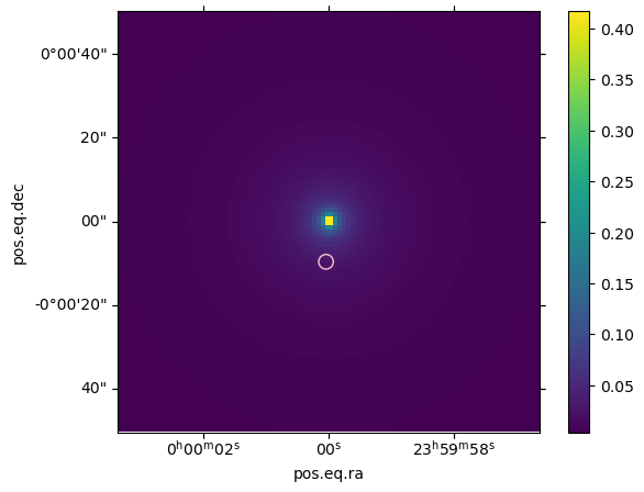
Here we have displayed the source in pink and the cluster of galaxies that acts as a lens in yellow. The colorbar indicates the mass repartition of the cluster in 10^{12} Msun/pixel.

Modelling gravitational lensing

Using the data from the above source, one or more images can be created corresponding to the gravitational lensing under study.

lt.e_lensing()
lt.get_images()

Compute multiple images for source 0...images found 3, not found 0

Table length=3

n	x	y	a	b	theta	z	mag
str2	float64	float64	float64	float64	float64	float64	float64
1a	-0.1439036032657953	2.0560154188542463	3.5000000009029875	0.7418610444825656	274.0036883033475	1.0	21.684363693981073
1a	-0.14387454674726022	2.057052271183944	3.500000000902991	0.7423114188365738	274.00087143112734	1.0	21.683704757410105
1a	1.5017408667543064	-21.45605858938671	7.741844354807153	3.5000000009029857	184.0036860228906	1.0	19.13805902100179

def plot_images():
    fig = plt.figure()
    ax = fig.add_axes([0.15, 0.1, 0.8, 0.8], projection=wcs)
    plt.imshow(mass)

    norm = Normalize(min(lt.get_images()['mag']), max(lt.get_images()['mag']))
    for row in lt.get_images(): 
        ellipse = Ellipse((row['x']/3600.,row['y']/3600.),
                          width=row['b']/3600,
                          height=row['a']/3600,
                          facecolor = 'none',
                          angle =row['theta'] + 90,
                          transform=plt.gca().get_transform('world')
                         )
         # Assign color to the ellipse based on the magnification

        color = cm.ScalarMappable(norm=norm, cmap = 'Wistia').to_rgba(row['mag'])
        ellipse.set_edgecolor(color)

        ax.add_patch(ellipse)

    # Creating a ScalarMappable object for colorbar
    cmap = cm.ScalarMappable(norm=norm, cmap = 'Wistia')
    cmap.set_array(tab['mag'])

    # Adding the colorbar
    colorbar = plt.colorbar(cmap)
    colorbar.set_label('Magnitude')
    plt.colorbar()
    plt.show()
plot_images()

/var/folders/mm/6xbl_6k14pn5zn23cltp9rzc0000gn/T/ipykernel_24111/310927048.py:27: MatplotlibDeprecationWarning: Unable to determine Axes to steal space for Colorbar. Using gca(), but will raise in the future. Either provide the *cax* argument to use as the Axes for the Colorbar, provide the *ax* argument to steal space from it, or add *mappable* to an Axes.
  colorbar = plt.colorbar(cmap)

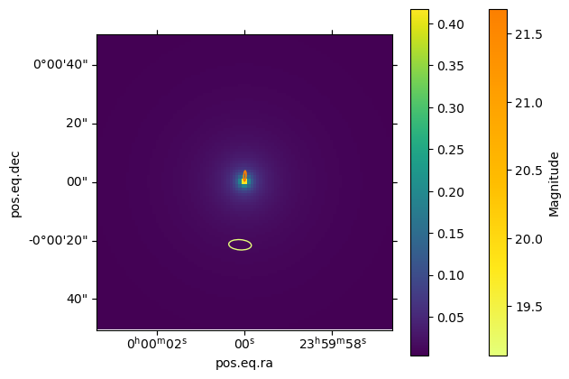
As we can see, three images are displayed whereas in the SIS model only two images should appear. This happens because due to numerical resolution limits, Lenstool finds two radial images, whereas only one should exist in theory. Note that depending on the grid.number, and grid.polar parameters, this third image is not always detected.

With another source

tab = Table(
    rows=[('1a', 10.6789067, 10.7, 3.5, 3.5, 0, 1.0, 20)],
    names=['n','x','y','a','b','theta','z','mag'], 
    dtype=['str',*['float',]*7]
)
lt.set_sources(tab)
lt.get_sources()

Table length=1

n	x	y	a	b	theta	z	mag
str2	float64	float64	float64	float64	float64	float64	float64
1a	10.6789067	10.7	3.5	3.5	0.0	1.0	20.0

lt.e_lensing()
display(lt.get_images())

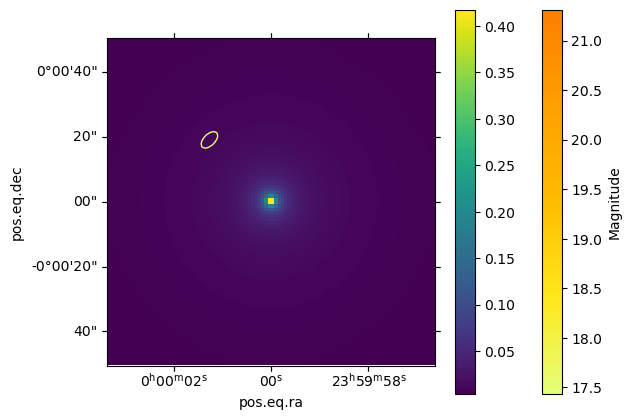
Compute multiple images for source 0...images found 1, not found 0

Table length=1

n	x	y	a	b	theta	z	mag
str2	float64	float64	float64	float64	float64	float64	float64
1a	19.003780153858134	19.041315591211987	6.228466685230651	3.5000000004546004	135.05652820048417	1.0	19.374217246134503

plot_images()

/var/folders/mm/6xbl_6k14pn5zn23cltp9rzc0000gn/T/ipykernel_24111/310927048.py:27: MatplotlibDeprecationWarning: Unable to determine Axes to steal space for Colorbar. Using gca(), but will raise in the future. Either provide the *cax* argument to use as the Axes for the Colorbar, provide the *ax* argument to steal space from it, or add *mappable* to an Axes.
  colorbar = plt.colorbar(cmap)

tab = Table(
    rows=[('1a', 1.7, 1.7, 3.5, 3.5, 0, 1.0, 20)],
    names=['n','x','y','a','b','theta','z','mag'], 
    dtype=['str',*['float',]*7]
)
lt.set_sources(tab)
lt.get_sources()

Table length=1

n	x	y	a	b	theta	z	mag
str2	float64	float64	float64	float64	float64	float64	float64
1a	1.7	1.7	3.5	3.5	0.0	1.0	20.0

lt.e_lensing()
display(lt.get_images())

Compute multiple images for source 0...images found 2, not found 0

Table length=2

n	x	y	a	b	theta	z	mag
str2	float64	float64	float64	float64	float64	float64	float64
1a	10.033094210747203	10.033094210747207	20.656397190255532	3.5000000004537077	134.99999999105756	1.0	18.072533671216917
1a	-6.6330663752945656	-6.6330663752945656	13.65607183861927	3.5000000004537037	134.99999999408797	1.0	18.521855628870078

plot_images()

/var/folders/mm/6xbl_6k14pn5zn23cltp9rzc0000gn/T/ipykernel_24111/310927048.py:27: MatplotlibDeprecationWarning: Unable to determine Axes to steal space for Colorbar. Using gca(), but will raise in the future. Either provide the *cax* argument to use as the Axes for the Colorbar, provide the *ax* argument to steal space from it, or add *mappable* to an Axes.
  colorbar = plt.colorbar(cmap)

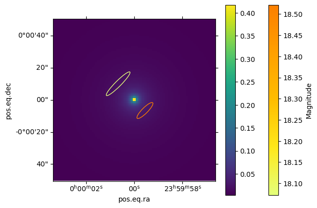
By moving the source closer to the lens, the flux can be amplified. The second colorbar represents the magnitude values of the obtained images.

tab = Table(
    rows=[('1a', 0.6789067, -9.7, 5.5, 5.5, 0, 1.5, 20)],
    names=['n','x','y','a','b','theta','z','mag'], 
    dtype=['str',*['float',]*7]
)
lt.set_sources(tab)
lt.get_sources()

Table length=1

n	x	y	a	b	theta	z	mag
str2	float64	float64	float64	float64	float64	float64	float64
1a	0.6789067	-9.7	5.5	5.5	0.0	1.5	20.0

lt.e_lensing()
display(lt.get_images())

Compute multiple images for source 0...images found 2, not found 0

Table length=2

n	x	y	a	b	theta	z	mag
str2	float64	float64	float64	float64	float64	float64	float64
1a	-0.25707791557222537	3.672954994000554	5.500000001342866	2.0826060496906016	94.00372378931525	1.5	21.054388909410584
1a	1.6149036200952676	-23.072957535127333	13.082585562250514	5.500000001342866	184.00367029497949	1.5	19.059172764025583

plot_images()

/var/folders/mm/6xbl_6k14pn5zn23cltp9rzc0000gn/T/ipykernel_24111/310927048.py:27: MatplotlibDeprecationWarning: Unable to determine Axes to steal space for Colorbar. Using gca(), but will raise in the future. Either provide the *cax* argument to use as the Axes for the Colorbar, provide the *ax* argument to steal space from it, or add *mappable* to an Axes.
  colorbar = plt.colorbar(cmap)

The image obtained for the first source studied is modelled again and the size of the source is increased; it can be seen that the size of the image is also increased.

tab = Table(
    rows=[('1a', 0.6789067, -9.7, 3.5, 3.5, 0, 15.0, 20)],
    names=['n','x','y','a','b','theta','z','mag'], 
    dtype=['str',*['float',]*7]
)
lt.set_sources(tab)
lt.get_sources()

Table length=1

n	x	y	a	b	theta	z	mag
str2	float64	float64	float64	float64	float64	float64	float64
1a	0.6789067	-9.7	3.5	3.5	0.0	15.0	20.0

lt.e_lensing()
display(lt.get_images())

Compute multiple images for source 0...images found 2, not found 0

Table length=2

n	x	y	a	b	theta	z	mag
str2	float64	float64	float64	float64	float64	float64	float64
1a	1.8173670426662405	-25.965958656690344	9.369170222656104	3.50000000232949	184.00362385225992	15.0	18.93091728652996
1a	-0.4595568468859513	6.565971489067192	3.50000000232949	2.369165693006243	274.0036418742858	15.0	20.423681522252945

plot_images()

/var/folders/mm/6xbl_6k14pn5zn23cltp9rzc0000gn/T/ipykernel_24111/310927048.py:27: MatplotlibDeprecationWarning: Unable to determine Axes to steal space for Colorbar. Using gca(), but will raise in the future. Either provide the *cax* argument to use as the Axes for the Colorbar, provide the *ax* argument to steal space from it, or add *mappable* to an Axes.
  colorbar = plt.colorbar(cmap)

When the redshift is increased, the distance between the images is also increased.

tab = Table(
    rows=[('1a', 0.3789067, 0.4, 3.5, 3.5, 0, 1.0, 20)],
    names=['n','x','y','a','b','theta','z','mag'], 
    dtype=['str',*['float',]*7]
)
lt.set_sources(tab)
lt.get_sources()

Table length=1

n	x	y	a	b	theta	z	mag
str2	float64	float64	float64	float64	float64	float64	float64
1a	0.3789067	0.4	3.5	3.5	0.0	1.0	20.0

lt.e_lensing()
display(lt.get_images())

Compute multiple images for source 0...images found 2, not found 0

Table length=2

n	x	y	a	b	theta	z	mag
str2	float64	float64	float64	float64	float64	float64	float64
1a	8.483351108269728	8.955704565242327	78.35533537154147	3.500000000478264	136.55153147905978	1.0	16.62499867624839
1a	-7.725506849912627	-8.155647694845774	71.35961784032642	3.500000000478264	136.5514760544116	1.0	16.726538821848983

plot_images()

/var/folders/mm/6xbl_6k14pn5zn23cltp9rzc0000gn/T/ipykernel_24111/310927048.py:27: MatplotlibDeprecationWarning: Unable to determine Axes to steal space for Colorbar. Using gca(), but will raise in the future. Either provide the *cax* argument to use as the Axes for the Colorbar, provide the *ax* argument to steal space from it, or add *mappable* to an Axes.
  colorbar = plt.colorbar(cmap)

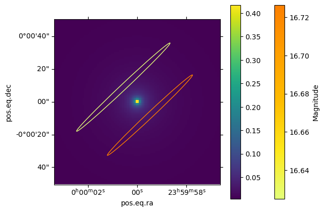
By moving the source closer to the lens again, the images appear streched.

Modelling of the Einstein ring

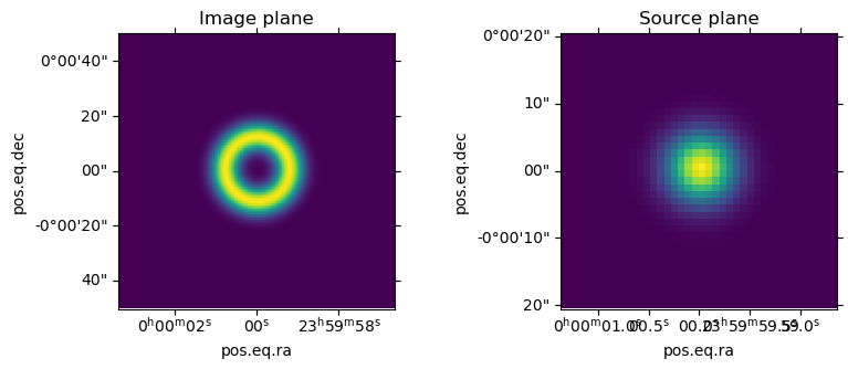
Now that we have seen the impact of each parameter on the resulting image, we want to model the Einstein ring. To do so we can model the brightness map with lenstool.

pix, wcs = lt.e_pixel_image(100)
source, swcs = lt.e_pixel_source(100)
fig = plt.figure(figsize=(10,5))
ax = fig.add_axes([0.15, 0.1, 0.5, 0.5], projection=wcs)

plt.imshow(pix)

ax.autoscale_view()
ax.set_title('Image plane')

ax = fig.add_axes([0.55, 0.1, 0.5, 0.5], projection=swcs)

plt.imshow(source)
ax.autoscale_view()
ax.set_title('Source plane')

image (100,100) s=1.010 [-50.000,50.000] [-50.000,50.000]

source (40,40) s=(1.026,1.026) [-20.000,20.000] [-20.000,20.000]

Text(0.5, 1.0, 'Source plane')

The convergence map

Lenstool can also compute the convergence map of the lens.

conv, wcs = lt.g_mass(1, 100, 0.3, 1.0)

fig = plt.figure()
ax = fig.add_axes([0.15, 0.1, 0.8, 0.8], projection=wcs)

s = abs(conv - 1/2) < 0.02
conv[s] = 10
plt.imshow(conv)
plt.colorbar()

<matplotlib.colorbar.Colorbar at 0x110517370>

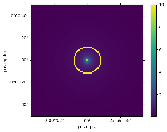
Here, the yellow circle is the critical line for our SIS model (when the convergence = 1/2).

Calculation of the Einstein ring

We start by using the lensing equations to obtain the radius of the ring created by gravitational lensing.
$\theta_{E} = \frac{4 \pi\sigma_{v}^{2}}{c^{2}}\frac{D_{LS}}{D_{S}}$

We can calculate the distances to the source and to the lens with the redshift data.

from math import pi
import astropy.constants as const
import astropy.units as u
from astropy.cosmology import FlatLambdaCDM

cosmo= FlatLambdaCDM(70,0.3)                     # definition of the universe (H0, z_lens)
dol=cosmo.angular_diameter_distance(0.3)         # distance between the observer and the lens
dos=cosmo.angular_diameter_distance(1)           # distance between the observer and the source
dls=cosmo.angular_diameter_distance_z1z2(0.3,1)  # distance between the lens and the source
sigma = 800 * u.km /u.s
theta = (4*pi*sigma**2*dls)/(dos*const.c**2)
theta = theta.to('m2/m2').value
print("the radius value is:",theta)                                  

the radius value is: 5.713423457351444e-05

Now that we have the radius we can display the ring.
To observe the match with the magnification map, it is also possible to directly display the ring on it.

ampli, wcs = lt.g_ampli(1, 100, 1.0)

fig = plt.figure()
ax = fig.add_axes([0.15, 0.1, 0.8, 0.8], projection=wcs)

plt.imshow(ampli)
plt.clim((-1,2))
plt.colorbar()

c = Circle((0,0),
           numpy.degrees(theta),
           edgecolor='pink',
           facecolor='none',
           linewidth=4,
           transform=ax.get_transform('world')
          )
           
        
ax.add_patch(c)
ax.set_title('Magnification map')

Text(0.5, 1.0, 'Magnification map')

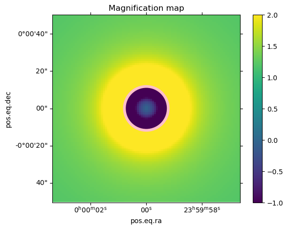
Here the Eistein ring is pink and the colorbar indicates the magnification factor.

Display of critical lines

Another method to represent the critical lines is to use the data calculated by Lenstool, we can then also represent the caustic lines.

from lenstool import pcl

# Compute image plane and source plane surface brightness maps
pix, wcs = lt.e_pixel_image(100)
source, swcs = lt.e_pixel_source(100)

# Compute critical and caustic external lines
tangent, radial = lt.criticnew(1.0)
critic_int, caustic_int = pcl.parse_cline(radial)

fig = plt.figure(figsize=(10,5))

ax = fig.add_axes([0.15, 0.1, 0.5, 0.5], projection=wcs)
plt.imshow(pix)
critic_int.set_transform(ax.get_transform('world'))
ax.add_collection(critic_int)
ax.autoscale_view()
ax.set_title('Image plane')

ax = fig.add_axes([0.55, 0.1, 0.5, 0.5], projection=swcs)
plt.imshow(source)
caustic_int.set_transform(ax.get_transform('world'))
ax.add_collection(caustic_int)
ax.autoscale_view()
ax.set_title('Source plane')

image (100,100) s=1.010 [-50.000,50.000] [-50.000,50.000]

source (40,40) s=(1.026,1.026) [-20.000,20.000] [-20.000,20.000]

COMP1: critic and caustic lines for source plane at z=1.000
limitHigh(in arcsec)=10.000 limitLow(in arcsec)=1.000

Text(0.5, 1.0, 'Source plane')

Here we display the external critical and caustic lines of the lens.
In the image plane, the critical line is a circle (as we calculated) superposed to the Einstein ring whereas the caustic line in the source plane is a point centered on the source.
If we were to model the internal lines, it would be the opposite, meaning that the internal critical line would be a point in the image plane and the caustic line a circle in the source plane. However, this point in the image plane is infinitely small, and Lenstool cannot find it, hence it cannot compute the associated caustic line.